
Rayleigh Taylor Instability with DualSPHysics5.0_NNewtonian

Hello DualSPHysics community! This is my first question on this forum.
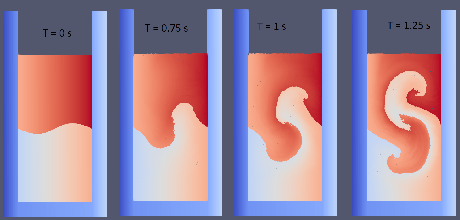
I am trying to reproduce a Rayleigh Tayler instability and I was relatively successful so far, but some uncertainties remain and maybe one of you can help me out. Above in the picture you can see what I have so far.
I have three questions:
1) In the multi-phase non-Newtonian examples of DualSPHysics the “VelocityGradientType” 1:FDA is always selected. What does FDA stand for? Can someone provide a source of documentation about this parameter?
2) Computing the pressure with the PartVTK tool of a multi-phase simulation gives an unexpected result. I expect a continuous pressure gradient increasing from top to bottom, resulting from the hydrostatic pressure. However, the result is different. there are pressure gradients from top to bottom but only within a single phase. What I observe is that both phases have a pressure gradient independently, but at different pressure levels (only visible when rescaled properly in paraview). There is not one continuous pressure gradient from top to bottom for both phases. Is this a result of the PartVTK tool simply converting the particle density into pressure via the state equation? Is there a different way to do it for a multi-phase simulation?
3) How do I lower the viscosity and still obtain a physical result? In my example I use kinematic viscosities for oil and water of about 10^-4. What I want is to reduce them to 10^-6. But doing this, the fluid expands after about 0.8 s and the particles will bounce around like crazy. I noticed unphysical density fluctuation (like oscillating numerical noise) just before this phenomena occurs. Therefore, I tested around with the density diffusion formulation of Molteni and Fourtakas, but nothing influenced my simulation, like absolutely zero difference. Is there a different way for me to implement a density diffusion formulation? And coming back to the original question, is there another way how to lower the viscosities?
thank you for developeing such a nice open source software!!
Debug Trace
| Notice |
rich is deprecated. Use FormatService::renderHtml($content, Formats\RichFormat::FORMAT_KEY) instead.

#0 [internal function]: gdn_ErrorHandler(16384, 'rich is depreca...', '/var/www/forums...', 950, Array)
#1 /var/www/forums-dual-sphysics-org/library/core/functions.general.php(950): trigger_error('rich is depreca...', 16384)
#2 /var/www/forums-dual-sphysics-org/library/core/class.format.php(1729): deprecated('rich', 'FormatService::...')
#3 /var/www/forums-dual-sphysics-org/library/core/class.format.php(1479): Gdn_Format::rich('[{"insert":{"em...')
#4 /var/www/forums-dual-sphysics-org/applications/vanilla/controllers/class.discussioncontroller.php(197): Gdn_Format::to('[{"insert":{"em...', 'Rich')
#5 /var/www/forums-dual-sphysics-org/applications/vanilla/controllers/class.discussioncontroller.php(402): DiscussionController->index(1848, 'x', 'p1')
#6 /var/www/forums-dual-sphysics-org/library/core/class.dispatcher.php(862): DiscussionController->comment('4093')
#7 /var/www/forums-dual-sphysics-org/library/core/class.dispatcher.php(279): Gdn_Dispatcher->dispatchController(Object(Gdn_Request), Array)
#8 /var/www/forums-dual-sphysics-org/index.php(29): Gdn_Dispatcher->dispatch()
#9 {main} |
| Notice |
rich is deprecated. Use FormatService::renderHtml($content, Formats\RichFormat::FORMAT_KEY) instead.

#0 [internal function]: gdn_ErrorHandler(16384, 'rich is depreca...', '/var/www/forums...', 950, Array)
#1 /var/www/forums-dual-sphysics-org/library/core/functions.general.php(950): trigger_error('rich is depreca...', 16384)
#2 /var/www/forums-dual-sphysics-org/library/core/class.format.php(1729): deprecated('rich', 'FormatService::...')
#3 /var/www/forums-dual-sphysics-org/library/core/class.format.php(1479): Gdn_Format::rich('[{"insert":{"em...')
#4 /var/www/forums-dual-sphysics-org/applications/vanilla/views/discussion/helper_functions.php(24): Gdn_Format::to('[{"insert":{"em...', 'Rich')
#5 /var/www/forums-dual-sphysics-org/applications/vanilla/views/discussion/discussion.php(89): formatBody(Object(stdClass))
#6 /var/www/forums-dual-sphysics-org/applications/vanilla/views/discussion/index.php(31): include('/var/www/forums...')
#7 /var/www/forums-dual-sphysics-org/library/core/class.controller.php(778): include('/var/www/forums...')
#8 /var/www/forums-dual-sphysics-org/library/core/class.controller.php(1382): Gdn_Controller->fetchView('', false, false)
#9 /var/www/forums-dual-sphysics-org/library/core/class.pluggable.php(217): Gdn_Controller->xRender()
#10 /var/www/forums-dual-sphysics-org/applications/vanilla/controllers/class.discussioncontroller.php(310): Gdn_Pluggable->__call('render', Array)
#11 /var/www/forums-dual-sphysics-org/applications/vanilla/controllers/class.discussioncontroller.php(402): DiscussionController->index(1848, 'x', 'p1')
#12 /var/www/forums-dual-sphysics-org/library/core/class.dispatcher.php(862): DiscussionController->comment('4093')
#13 /var/www/forums-dual-sphysics-org/library/core/class.dispatcher.php(279): Gdn_Dispatcher->dispatchController(Object(Gdn_Request), Array)
#14 /var/www/forums-dual-sphysics-org/index.php(29): Gdn_Dispatcher->dispatch()
#15 {main} |
| Notice |
rich is deprecated. Use FormatService::renderHtml($content, Formats\RichFormat::FORMAT_KEY) instead.

#0 [internal function]: gdn_ErrorHandler(16384, 'rich is depreca...', '/var/www/forums...', 950, Array)
#1 /var/www/forums-dual-sphysics-org/library/core/functions.general.php(950): trigger_error('rich is depreca...', 16384)
#2 /var/www/forums-dual-sphysics-org/library/core/class.format.php(1729): deprecated('rich', 'FormatService::...')
#3 /var/www/forums-dual-sphysics-org/library/core/class.format.php(1479): Gdn_Format::rich('[{"insert":{"em...')
#4 /var/www/forums-dual-sphysics-org/applications/vanilla/views/discussion/helper_functions.php(24): Gdn_Format::to('[{"insert":{"em...', 'Rich')
#5 /var/www/forums-dual-sphysics-org/applications/vanilla/views/discussion/helper_functions.php(170): formatBody(Object(stdClass))
#6 /var/www/forums-dual-sphysics-org/applications/vanilla/views/discussion/comments.php(19): writeComment(Object(stdClass), Object(DiscussionController), Object(Gdn_Session), 1)
#7 /var/www/forums-dual-sphysics-org/applications/vanilla/views/discussion/index.php(53): include('/var/www/forums...')
#8 /var/www/forums-dual-sphysics-org/library/core/class.controller.php(778): include('/var/www/forums...')
#9 /var/www/forums-dual-sphysics-org/library/core/class.controller.php(1382): Gdn_Controller->fetchView('', false, false)
#10 /var/www/forums-dual-sphysics-org/library/core/class.pluggable.php(217): Gdn_Controller->xRender()
#11 /var/www/forums-dual-sphysics-org/applications/vanilla/controllers/class.discussioncontroller.php(310): Gdn_Pluggable->__call('render', Array)
#12 /var/www/forums-dual-sphysics-org/applications/vanilla/controllers/class.discussioncontroller.php(402): DiscussionController->index(1848, 'x', 'p1')
#13 /var/www/forums-dual-sphysics-org/library/core/class.dispatcher.php(862): DiscussionController->comment('4093')
#14 /var/www/forums-dual-sphysics-org/library/core/class.dispatcher.php(279): Gdn_Dispatcher->dispatchController(Object(Gdn_Request), Array)
#15 /var/www/forums-dual-sphysics-org/index.php(29): Gdn_Dispatcher->dispatch()
#16 {main} |
| Notice |
rich is deprecated. Use FormatService::renderHtml($content, Formats\RichFormat::FORMAT_KEY) instead.

#0 [internal function]: gdn_ErrorHandler(16384, 'rich is depreca...', '/var/www/forums...', 950, Array)
#1 /var/www/forums-dual-sphysics-org/library/core/functions.general.php(950): trigger_error('rich is depreca...', 16384)
#2 /var/www/forums-dual-sphysics-org/library/core/class.format.php(1729): deprecated('rich', 'FormatService::...')
#3 /var/www/forums-dual-sphysics-org/library/core/class.format.php(1479): Gdn_Format::rich('[{"insert":"Hi ...')
#4 /var/www/forums-dual-sphysics-org/applications/vanilla/views/discussion/helper_functions.php(24): Gdn_Format::to('[{"insert":"Hi ...', 'Rich')
#5 /var/www/forums-dual-sphysics-org/applications/vanilla/views/discussion/helper_functions.php(170): formatBody(Object(stdClass))
#6 /var/www/forums-dual-sphysics-org/applications/vanilla/views/discussion/comments.php(19): writeComment(Object(stdClass), Object(DiscussionController), Object(Gdn_Session), 2)
#7 /var/www/forums-dual-sphysics-org/applications/vanilla/views/discussion/index.php(53): include('/var/www/forums...')
#8 /var/www/forums-dual-sphysics-org/library/core/class.controller.php(778): include('/var/www/forums...')
#9 /var/www/forums-dual-sphysics-org/library/core/class.controller.php(1382): Gdn_Controller->fetchView('', false, false)
#10 /var/www/forums-dual-sphysics-org/library/core/class.pluggable.php(217): Gdn_Controller->xRender()
#11 /var/www/forums-dual-sphysics-org/applications/vanilla/controllers/class.discussioncontroller.php(310): Gdn_Pluggable->__call('render', Array)
#12 /var/www/forums-dual-sphysics-org/applications/vanilla/controllers/class.discussioncontroller.php(402): DiscussionController->index(1848, 'x', 'p1')
#13 /var/www/forums-dual-sphysics-org/library/core/class.dispatcher.php(862): DiscussionController->comment('4093')
#14 /var/www/forums-dual-sphysics-org/library/core/class.dispatcher.php(279): Gdn_Dispatcher->dispatchController(Object(Gdn_Request), Array)
#15 /var/www/forums-dual-sphysics-org/index.php(29): Gdn_Dispatcher->dispatch()
#16 {main} |
| Notice |
rich is deprecated. Use FormatService::renderHtml($content, Formats\RichFormat::FORMAT_KEY) instead.

#0 [internal function]: gdn_ErrorHandler(16384, 'rich is depreca...', '/var/www/forums...', 950, Array)
#1 /var/www/forums-dual-sphysics-org/library/core/functions.general.php(950): trigger_error('rich is depreca...', 16384)
#2 /var/www/forums-dual-sphysics-org/library/core/class.format.php(1729): deprecated('rich', 'FormatService::...')
#3 /var/www/forums-dual-sphysics-org/library/core/class.format.php(1479): Gdn_Format::rich('[{"insert":"Tha...')
#4 /var/www/forums-dual-sphysics-org/applications/vanilla/views/discussion/helper_functions.php(24): Gdn_Format::to('[{"insert":"Tha...', 'Rich')
#5 /var/www/forums-dual-sphysics-org/applications/vanilla/views/discussion/helper_functions.php(170): formatBody(Object(stdClass))
#6 /var/www/forums-dual-sphysics-org/applications/vanilla/views/discussion/comments.php(19): writeComment(Object(stdClass), Object(DiscussionController), Object(Gdn_Session), 3)
#7 /var/www/forums-dual-sphysics-org/applications/vanilla/views/discussion/index.php(53): include('/var/www/forums...')
#8 /var/www/forums-dual-sphysics-org/library/core/class.controller.php(778): include('/var/www/forums...')
#9 /var/www/forums-dual-sphysics-org/library/core/class.controller.php(1382): Gdn_Controller->fetchView('', false, false)
#10 /var/www/forums-dual-sphysics-org/library/core/class.pluggable.php(217): Gdn_Controller->xRender()
#11 /var/www/forums-dual-sphysics-org/applications/vanilla/controllers/class.discussioncontroller.php(310): Gdn_Pluggable->__call('render', Array)
#12 /var/www/forums-dual-sphysics-org/applications/vanilla/controllers/class.discussioncontroller.php(402): DiscussionController->index(1848, 'x', 'p1')
#13 /var/www/forums-dual-sphysics-org/library/core/class.dispatcher.php(862): DiscussionController->comment('4093')
#14 /var/www/forums-dual-sphysics-org/library/core/class.dispatcher.php(279): Gdn_Dispatcher->dispatchController(Object(Gdn_Request), Array)
#15 /var/www/forums-dual-sphysics-org/index.php(29): Gdn_Dispatcher->dispatch()
#16 {main} |
| Notice |
rich is deprecated. Use FormatService::renderHtml($content, Formats\RichFormat::FORMAT_KEY) instead.

#0 [internal function]: gdn_ErrorHandler(16384, 'rich is depreca...', '/var/www/forums...', 950, Array)
#1 /var/www/forums-dual-sphysics-org/library/core/functions.general.php(950): trigger_error('rich is depreca...', 16384)
#2 /var/www/forums-dual-sphysics-org/library/core/class.format.php(1729): deprecated('rich', 'FormatService::...')
#3 /var/www/forums-dual-sphysics-org/library/core/class.format.php(1479): Gdn_Format::rich('[{"insert":"I w...')
#4 /var/www/forums-dual-sphysics-org/applications/vanilla/views/discussion/helper_functions.php(24): Gdn_Format::to('[{"insert":"I w...', 'Rich')
#5 /var/www/forums-dual-sphysics-org/applications/vanilla/views/discussion/helper_functions.php(170): formatBody(Object(stdClass))
#6 /var/www/forums-dual-sphysics-org/applications/vanilla/views/discussion/comments.php(19): writeComment(Object(stdClass), Object(DiscussionController), Object(Gdn_Session), 4)
#7 /var/www/forums-dual-sphysics-org/applications/vanilla/views/discussion/index.php(53): include('/var/www/forums...')
#8 /var/www/forums-dual-sphysics-org/library/core/class.controller.php(778): include('/var/www/forums...')
#9 /var/www/forums-dual-sphysics-org/library/core/class.controller.php(1382): Gdn_Controller->fetchView('', false, false)
#10 /var/www/forums-dual-sphysics-org/library/core/class.pluggable.php(217): Gdn_Controller->xRender()
#11 /var/www/forums-dual-sphysics-org/applications/vanilla/controllers/class.discussioncontroller.php(310): Gdn_Pluggable->__call('render', Array)
#12 /var/www/forums-dual-sphysics-org/applications/vanilla/controllers/class.discussioncontroller.php(402): DiscussionController->index(1848, 'x', 'p1')
#13 /var/www/forums-dual-sphysics-org/library/core/class.dispatcher.php(862): DiscussionController->comment('4093')
#14 /var/www/forums-dual-sphysics-org/library/core/class.dispatcher.php(279): Gdn_Dispatcher->dispatchController(Object(Gdn_Request), Array)
#15 /var/www/forums-dual-sphysics-org/index.php(29): Gdn_Dispatcher->dispatch()
#16 {main} |
| Notice |
rich is deprecated. Use FormatService::renderHtml($content, Formats\RichFormat::FORMAT_KEY) instead.

#0 [internal function]: gdn_ErrorHandler(16384, 'rich is depreca...', '/var/www/forums...', 950, Array)
#1 /var/www/forums-dual-sphysics-org/library/core/functions.general.php(950): trigger_error('rich is depreca...', 16384)
#2 /var/www/forums-dual-sphysics-org/library/core/class.format.php(1729): deprecated('rich', 'FormatService::...')
#3 /var/www/forums-dual-sphysics-org/library/core/class.format.php(1479): Gdn_Format::rich('[{"insert":"Abo...')
#4 /var/www/forums-dual-sphysics-org/applications/vanilla/views/discussion/helper_functions.php(24): Gdn_Format::to('[{"insert":"Abo...', 'Rich')
#5 /var/www/forums-dual-sphysics-org/applications/vanilla/views/discussion/helper_functions.php(170): formatBody(Object(stdClass))
#6 /var/www/forums-dual-sphysics-org/applications/vanilla/views/discussion/comments.php(19): writeComment(Object(stdClass), Object(DiscussionController), Object(Gdn_Session), 5)
#7 /var/www/forums-dual-sphysics-org/applications/vanilla/views/discussion/index.php(53): include('/var/www/forums...')
#8 /var/www/forums-dual-sphysics-org/library/core/class.controller.php(778): include('/var/www/forums...')
#9 /var/www/forums-dual-sphysics-org/library/core/class.controller.php(1382): Gdn_Controller->fetchView('', false, false)
#10 /var/www/forums-dual-sphysics-org/library/core/class.pluggable.php(217): Gdn_Controller->xRender()
#11 /var/www/forums-dual-sphysics-org/applications/vanilla/controllers/class.discussioncontroller.php(310): Gdn_Pluggable->__call('render', Array)
#12 /var/www/forums-dual-sphysics-org/applications/vanilla/controllers/class.discussioncontroller.php(402): DiscussionController->index(1848, 'x', 'p1')
#13 /var/www/forums-dual-sphysics-org/library/core/class.dispatcher.php(862): DiscussionController->comment('4093')
#14 /var/www/forums-dual-sphysics-org/library/core/class.dispatcher.php(279): Gdn_Dispatcher->dispatchController(Object(Gdn_Request), Array)
#15 /var/www/forums-dual-sphysics-org/index.php(29): Gdn_Dispatcher->dispatch()
#16 {main} |
| Notice |
rich is deprecated. Use FormatService::renderHtml($content, Formats\RichFormat::FORMAT_KEY) instead.

#0 [internal function]: gdn_ErrorHandler(16384, 'rich is depreca...', '/var/www/forums...', 950, Array)
#1 /var/www/forums-dual-sphysics-org/library/core/functions.general.php(950): trigger_error('rich is depreca...', 16384)
#2 /var/www/forums-dual-sphysics-org/library/core/class.format.php(1729): deprecated('rich', 'FormatService::...')
#3 /var/www/forums-dual-sphysics-org/library/core/class.format.php(1479): Gdn_Format::rich('[{"insert":"Hi ...')
#4 /var/www/forums-dual-sphysics-org/applications/vanilla/views/discussion/helper_functions.php(24): Gdn_Format::to('[{"insert":"Hi ...', 'Rich')
#5 /var/www/forums-dual-sphysics-org/applications/vanilla/views/discussion/helper_functions.php(170): formatBody(Object(stdClass))
#6 /var/www/forums-dual-sphysics-org/applications/vanilla/views/discussion/comments.php(19): writeComment(Object(stdClass), Object(DiscussionController), Object(Gdn_Session), 6)
#7 /var/www/forums-dual-sphysics-org/applications/vanilla/views/discussion/index.php(53): include('/var/www/forums...')
#8 /var/www/forums-dual-sphysics-org/library/core/class.controller.php(778): include('/var/www/forums...')
#9 /var/www/forums-dual-sphysics-org/library/core/class.controller.php(1382): Gdn_Controller->fetchView('', false, false)
#10 /var/www/forums-dual-sphysics-org/library/core/class.pluggable.php(217): Gdn_Controller->xRender()
#11 /var/www/forums-dual-sphysics-org/applications/vanilla/controllers/class.discussioncontroller.php(310): Gdn_Pluggable->__call('render', Array)
#12 /var/www/forums-dual-sphysics-org/applications/vanilla/controllers/class.discussioncontroller.php(402): DiscussionController->index(1848, 'x', 'p1')
#13 /var/www/forums-dual-sphysics-org/library/core/class.dispatcher.php(862): DiscussionController->comment('4093')
#14 /var/www/forums-dual-sphysics-org/library/core/class.dispatcher.php(279): Gdn_Dispatcher->dispatchController(Object(Gdn_Request), Array)
#15 /var/www/forums-dual-sphysics-org/index.php(29): Gdn_Dispatcher->dispatch()
#16 {main} |
| Notice |
rich is deprecated. Use FormatService::renderHtml($content, Formats\RichFormat::FORMAT_KEY) instead.

#0 [internal function]: gdn_ErrorHandler(16384, 'rich is depreca...', '/var/www/forums...', 950, Array)
#1 /var/www/forums-dual-sphysics-org/library/core/functions.general.php(950): trigger_error('rich is depreca...', 16384)
#2 /var/www/forums-dual-sphysics-org/library/core/class.format.php(1729): deprecated('rich', 'FormatService::...')
#3 /var/www/forums-dual-sphysics-org/library/core/class.format.php(1479): Gdn_Format::rich('[{"insert":"Tha...')
#4 /var/www/forums-dual-sphysics-org/applications/vanilla/views/discussion/helper_functions.php(24): Gdn_Format::to('[{"insert":"Tha...', 'Rich')
#5 /var/www/forums-dual-sphysics-org/applications/vanilla/views/discussion/helper_functions.php(170): formatBody(Object(stdClass))
#6 /var/www/forums-dual-sphysics-org/applications/vanilla/views/discussion/comments.php(19): writeComment(Object(stdClass), Object(DiscussionController), Object(Gdn_Session), 7)
#7 /var/www/forums-dual-sphysics-org/applications/vanilla/views/discussion/index.php(53): include('/var/www/forums...')
#8 /var/www/forums-dual-sphysics-org/library/core/class.controller.php(778): include('/var/www/forums...')
#9 /var/www/forums-dual-sphysics-org/library/core/class.controller.php(1382): Gdn_Controller->fetchView('', false, false)
#10 /var/www/forums-dual-sphysics-org/library/core/class.pluggable.php(217): Gdn_Controller->xRender()
#11 /var/www/forums-dual-sphysics-org/applications/vanilla/controllers/class.discussioncontroller.php(310): Gdn_Pluggable->__call('render', Array)
#12 /var/www/forums-dual-sphysics-org/applications/vanilla/controllers/class.discussioncontroller.php(402): DiscussionController->index(1848, 'x', 'p1')
#13 /var/www/forums-dual-sphysics-org/library/core/class.dispatcher.php(862): DiscussionController->comment('4093')
#14 /var/www/forums-dual-sphysics-org/library/core/class.dispatcher.php(279): Gdn_Dispatcher->dispatchController(Object(Gdn_Request), Array)
#15 /var/www/forums-dual-sphysics-org/index.php(29): Gdn_Dispatcher->dispatch()
#16 {main} |
| Notice |
rich is deprecated. Use FormatService::renderHtml($content, Formats\RichFormat::FORMAT_KEY) instead.

#0 [internal function]: gdn_ErrorHandler(16384, 'rich is depreca...', '/var/www/forums...', 950, Array)
#1 /var/www/forums-dual-sphysics-org/library/core/functions.general.php(950): trigger_error('rich is depreca...', 16384)
#2 /var/www/forums-dual-sphysics-org/library/core/class.format.php(1729): deprecated('rich', 'FormatService::...')
#3 /var/www/forums-dual-sphysics-org/library/core/class.format.php(1479): Gdn_Format::rich('[{"insert":"I a...')
#4 /var/www/forums-dual-sphysics-org/applications/vanilla/views/discussion/helper_functions.php(24): Gdn_Format::to('[{"insert":"I a...', 'Rich')
#5 /var/www/forums-dual-sphysics-org/applications/vanilla/views/discussion/helper_functions.php(170): formatBody(Object(stdClass))
#6 /var/www/forums-dual-sphysics-org/applications/vanilla/views/discussion/comments.php(19): writeComment(Object(stdClass), Object(DiscussionController), Object(Gdn_Session), 8)
#7 /var/www/forums-dual-sphysics-org/applications/vanilla/views/discussion/index.php(53): include('/var/www/forums...')
#8 /var/www/forums-dual-sphysics-org/library/core/class.controller.php(778): include('/var/www/forums...')
#9 /var/www/forums-dual-sphysics-org/library/core/class.controller.php(1382): Gdn_Controller->fetchView('', false, false)
#10 /var/www/forums-dual-sphysics-org/library/core/class.pluggable.php(217): Gdn_Controller->xRender()
#11 /var/www/forums-dual-sphysics-org/applications/vanilla/controllers/class.discussioncontroller.php(310): Gdn_Pluggable->__call('render', Array)
#12 /var/www/forums-dual-sphysics-org/applications/vanilla/controllers/class.discussioncontroller.php(402): DiscussionController->index(1848, 'x', 'p1')
#13 /var/www/forums-dual-sphysics-org/library/core/class.dispatcher.php(862): DiscussionController->comment('4093')
#14 /var/www/forums-dual-sphysics-org/library/core/class.dispatcher.php(279): Gdn_Dispatcher->dispatchController(Object(Gdn_Request), Array)
#15 /var/www/forums-dual-sphysics-org/index.php(29): Gdn_Dispatcher->dispatch()
#16 {main} |
Comments
Here is the used xml code, if it helps someone make more sense of my questions.
Hi Hannes
1.
DualSPHysics_v5.0/doc/guides/XML_GUIDE_MPHASE_NNEWTONIAN.pdf
This is FDA as far as I understand
2. would be nice with some plots, I think what you describe could be the issue. Try testing in Paraview using the SPH Line Interpolation tool.
3. Perhaps you need to play with some of the other parameters like tau when changing viscosities
Kind regards
Thank you for your response, I appreciate your help!
1) FDA = Finite Differences approach, ok.
2) I show you what I mean with plots. The result of the single phase simulation plotting the pressure with the SPH line interpolation tool gives:
This is a somewhat expected result, the pressure decreases from 1.5 bar down to 0 from bottom to top. If I do the same procedure for a multi-phase simulation the result is this:
The pressure does not behave in a physical way (it is below 0 between position 7000 and 9000 on the z axys in the plot and makes huge jumps). In the render view you can see a pressure gradient on the upper fluid, because I rescaled the pressure accordingly between 1 bar and 1.1 bar in the paraview color map editor. Do you get the same result when plotting the pressure of a multi-phase simulation, or is there something else to consider compared to the single phase?
3) I made the same simulation now for different values of tau (0; 0.0005; 0.05 and 0.5). No difference can be made in the oscilatory behavior of the density. Here is a picture of what is going on:
The density is color coded according to the upper fluid. On the left side you see the density after 30 ms. The right side shows the same simulation after 70 ms.
Kind regards
I will be honest and say I do not understand how it seems to behave "visually correct" if the pressure is wrong.. I think maybe we are analyzing it wrongly? But I am not sure of course.
If I remember correctly the pressure formulation for single and multi-phase is different, have a look at the documentation, maybe that is where the issue lies.
I really like you are trying to do this kind of case, I also tried to do it a few years ago, but at the time I couldn't get it to be stable - yours is much closer!
Kind regards
About the pressure gradient: Yes exactly. The pressure seems to be correct in the render view but is completely off in the plot with the SPH Line interpolation tool. It is strange because the same procedure works for a single-phase simulation. Yes, maybe we are missing a point here.
About the density fluctuations: Note, that this behavior (last picture) only occurs when the viscosity of the two fluids is below 10^-4, otherwise it is stable (see header picture). My first intuition was to try out density diffusion formulations/DSPH variants, but none seem to have an influence. It would be nice to know if someone has experience with the density diffusion formulations together with multi-phase DualSPHysics5.0_NNewtonian simulations.
Kind regards
Hi Hannes,
On your questions:
1) FDA stands for finite differences approach. This approach uses a simple FD to calculate the velocity gradients and in turn all other summations are performed with an SPH summation. The reason we use the FDA approach in the example is because it is faster than the SPH velocity gradient calculation. Also, there are some theoretical matters which, I will not go into detail here.
2) As you said on the post above, using the measure tool gives you the "correct result" however the Paraview build-in tools does not. This depends on what your properties are, i,.e the density of each phase and derived from that your mass. Do not expect to get the correct results with the Paraview tool (although possible)
3) that is a difficult one, for a kinematic viscosity which is as low as 10^-6 the SPH scheme (and this is in general not just this implementation) may go unstable (fluctuations) as there is not enough diffusion to damp down the numerical error. A quick fix is to include very little artificial viscosity (on top of your kinematic) to filter out the noise. Remember that the artificial viscosity is simply a high frequency noise filter as used in FDs. Did the DDT1 or 2 help with the density fluctuations?
Your results in the first post look nice, any comparisons with known solutions?
Thanks,
George
Thank you for your response, this information is very valuable for me!
For now I could not recognize any effect on the density fluctuations from the DDT formulations 1, 2, or 3. This might be a problem of the finetuning of the DensityDTvalue and/or the fact, that a viscosity of 10^-6 is just too small to be reasonably handled by SPH. I will try to change the DDT configuration and see how the density stability behaves for different viscosities in order to figure out its effects.
My results are visually in close agreement with the results from Grenier et al 2009 (https://doi.org/10.1016/j.jcp.2009.08.009 ) and Hu & Adams 2007 (https://doi.org/10.1016/j.jcp.2007.07.013 ), which is also where I adopted the geometry from.
I am coming back to this post, since a relevant idea was proposed that may help me with a new project. Two posts above gfourtakas hinted to use a small amount of artificial viscosity on top of an already existing Laminar+SPS to limit oscillatory behaviour (answer 3). My question now is, how can I implement this? Is it possible to introduce both kinds of viscosity treatments from the _Def.xml file?
There is no case example doing this (as far as I am aware of), so I am unsure about how to enforce both viscosity formulations.
Regards,
Hannes